Why Any Distribution-Free Lower-Bound Estimator for Mutual Information Can’t Beat log N

A short explanation of McAllester & Stratos’ (2020) mututal information estimation result plus some intuition.

1. Background & Motivation

Mutual information (MI) plays a central role in information theory, communication theory and modern representation learning. Recent advances in neural networks, and the easier realisation of variational results for practical applications led to a rejuvenation of old representations of Kullback-Leibler divergence, i.e., the Donsker-Varadhan (DV) based lower bound, which was investigated in MINE (Mutual Information Neural Estimation) ¹.

Also other lower bounds for mutual information got renewed interest such as the Nguyien-Wainwright-Jordan (NWJ) lower bound ², and the more recent noise-contrastive method, the InfoNCE ³. In representation learning, these estimators can be used to learn from maximizing feature information in data. In communication theory, these estimators can be used to learn, for example, optimal encoding ⁴. I refer to the overview paper by Poole et al. ⁵ for a comprehensive overview.

All these recent bounds rely on lower bounds of mutual information estimated from finite samples. Formally, given a sample of size $N$, the algorithm computes a bound $\widehat I_{\mathrm{LB}} \le I(X;Y)$, hoping that it gets close to the true value, by approximating from below.

However, in practice the bounds linke MINE, NWJ and others exhibit high variance, and estimates fluctuate below AND above the true MI value, seemingly contradicting the theoretical results. The InfoNCE bound exhibits very low variance, but its MI value is limited to $\log N$, where $N$ is the batch size.

[Note that Poole et al. already showed that using Monte-Carlo approximation of the expectation terms in MINE, i.e. $\mathbb{E}_{p_{XY}}[f_\theta(X,Y)]- \log \mathbb{E}_{p_X p_Y}\!\bigl[e^{f_\theta(X,Y)}\bigr]$, yields neither a lower nor an upper bound due to the nonlinearity (log).]

McAllester and Stratos (2020) showed that this behavior is an inherent limitation. If an estimator is required to work on arbitrary distributions (i.e., “distribution-free”) and to provide valid lower bounds with high probability (say, with confidence $1 - \delta$), then it cannot exceed a constant times $\log N$. In other words, no universal, high-confidence lower bound can grow faster than logarithmically in the sample size.

2. Intuition — (Hidden Spikes in Data)

2.1 The discrete case

Lets have a look at a uniform distribution, which maximizes the entropy. We know that $I(X;Y) = H(X) - H(X|Y) \le H(X)$. Therefore MI is a lower bound for entropy. Given a finite support interval, the uniform distribution maximizes the entropy. Any spike in this distribution lowers the entropy. So the sampling mechanism needs to hit the spike, to accurately estimate the entropy. As the entropy upper bounds the MI, it can be seen how this problem directly translates to MI.

2.2 The continues case

Note. For continuous variables, the uniform density on a finite interval ([a,b]) still maximises differential entropy,
but (h(X)) itself can be negative. Consequently, the shortcut (I(X;Y)\le h(X)) that worked in the discrete case no longer provides a useful upper bound on mutual information and the proof must instead rely on the KL–divergence formulation.

To see why the $\log N$ ceiling is unavoidable, consider a simple trick an adversary can play on your data.

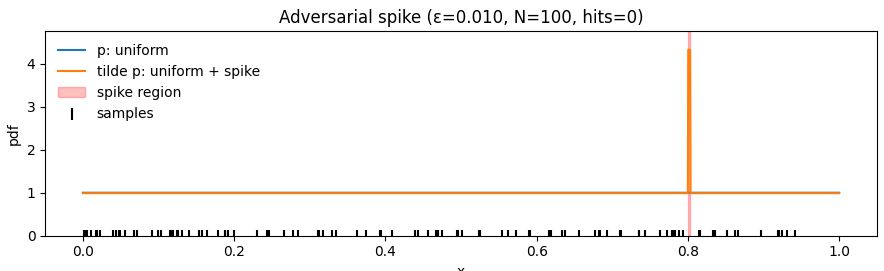
Start with a nice, well-behaved distribution $p(x)$. Now define a new distribution $\tilde{p}(x)$ that’s almost identical to $p$, except it hides a tiny spike $s(x)$:

where $s(x)$ is sharply concentrated on a narrow region. This spike carries just $1/N$ of the total probability mass.

Now sample $N$ points from $\tilde{p}$. With probability $(1-\frac{1}{N})^N$, the sample never hits the spike so the sample is indistinguishable from one drawn from $p$. For $N=2$ this is $1/4$, converging to $e^{-1}$ for $N\rightarrow \infty$. Yet, the spike can drastically lower the entropy, KL divergence, or mutual information of the true distribution, as argued above.

2.3 Sketch of the $\log N$ bound (KL Version)

In the case of KL divergence we have the following.

Suppose you want to estimate $D_{\mathrm{KL}}(p \Vert q)$ from a finite sample $S \sim p^N$, and your estimator $E(S)$ is required to be a high-confidence lower bound. That is, it must satisfy

Now imagine we have the same adversary as above, which modifies $q$ slightly by mixing in a bit of $p$, creating a new distribution:

This change guarantees that $\tilde{q}(x) \ge \frac{1}{N} p(x)$, and from this, it follows that

$\frac{p(x)}{\tilde{q}(x)}\le N$ and therefore $\mathbb{E}_{p}[\log \frac{p(x)}{\tilde{q}(x)}]\le \log N$ which is

At the same time, a batch of $N$ samples from $p$ is statistically very unlikely to detect the difference between $q$ and $\tilde{q}$, since the mass added to $p$ is only $1/N$. In fact, samples from $\tilde{q}^N$ and $q^N$ are nearly indistinguishable unless one of them lands in the spike, which happens with low probability. In fact, as argued above, the chance for this is greater than $1/4$.

So, if the estimator ever outputs a value greater than $\log N$ on a batch that looks like it came from $q$, it risks being wrong under $\tilde{q}$ with nontrivial probability ($e^{-1}$ in the limit) which is violating the confidence guarantee.

The safest strategy for the estimator is to stay below $\log N + \text{const}$, regardless of the true KL unless it has specific structural properties. Since mutual information is itself a KL divergence, this same limitation applies directly to MI lower bounds as well.

3 Lessons

• Without strong assumptions (finite alphabet, parametric family, smoothness), large lower bounds are impossible.

4 Refs

Mutual Information Neural Estimation (MINE).
Proceedings of the 35th International Conference on Machine Learning.

Estimating Divergence Functionals and the Likelihood Ratio by Convex Risk Minimization.
IEEE Transactions on Information Theory, 56 (11), 5847-5861.

Noise-Contrastive Estimation: A New Estimation Principle for Unnormalized Statistical Models.
In Proceedings of AISTATS 13, 297-304.

Deep Learning for Channel Coding via Neural Mutual Information Estimation.
In Proceedings of the 2019 IEEE 20th International Workshop on Signal Processing Advances in Wireless Communications (SPAWC), 1-5.

  On Variational Bounds of Mutual Information.
In Proceedings of the 36th International Conference on Machine Learning (ICML), 5171-5180.

5 Code and Visualization

 
import numpy as np
import matplotlib.pyplot as plt

# ----------------  parameters ---------------------
N     = 100      # batch size
eps   = 1/N      # hidden mass
width = 0.003    # spike width
pos   = 0.8      # spike start (interval [pos, pos+width])
# --------------------------------------------------

# pdfs on [0,1]
x     = np.linspace(0, 1, 2000)
p_pdf = np.ones_like(x)
q_pdf = np.ones_like(x)*(1-eps)
q_pdf += ((x>=pos) & (x<=pos+width)) * (eps/width)

# draw N samples from q_pdf (simple rejection sampler)
rng   = np.random.default_rng(42)
samps = []
while len(samps) < N:
    u = rng.random()
    if rng.random() <= q_pdf[(np.abs(x-u)<1e-3)][0] / q_pdf.max():
        samps.append(u)
samps = np.array(samps)

# count spike hits
hits = np.sum((samps >= pos) & (samps <= pos + width))
print(f"Spike hits: {hits} / {N}")

# plot
plt.figure(figsize=(9,3))
plt.plot(x, p_pdf, label='p: uniform')
plt.plot(x, q_pdf, label='tilde p: uniform + spike')
plt.axvspan(pos, pos + width, color='red', alpha=0.25, label='spike region')
plt.scatter(samps, np.zeros_like(samps), marker='|', s=80, color='k', label='samples')
plt.ylim(0, q_pdf.max()*1.1)
plt.xlabel('x'); plt.ylabel('pdf')
plt.title(f'Adversarial spike (ε={eps:.3f}, N={N}, hits={hits})')
plt.legend(frameon=False); plt.tight_layout()
plt.savefig('adversarial_spike.png', dpi=150)
plt.show()
```